Understand the result

What each number means, and when two numbers may be compared.

Wall time

Elapsed clock time across the measured operation, including any waiting inside it.

• The workload definition decides the boundary. Read it before interpreting a timing.

• Units: 1 s = 1,000 ms = 1,000,000 µs = 1,000,000,000 ns.

• CPU time counts processor execution. Threads consume it in parallel, and waiting uses none.

Samples and distributions

• A sample is one measured execution (or a batch normalized per evaluation).

• samples is how many to collect; evals is evaluations per sample.

• median — middle value; the usual summary.

• minimum — fastest observed.

• mean — sensitive to slow samples.

• p95 / p99 — thresholds covering about 95% / 99% of observations.

A small microbenchmark does not establish a production p99. That needs production-like input, concurrency and load.

Allocations and memory

• Allocated bytes — memory obtained during the operation.

• Allocation count — how many allocation events occurred.

• Live memory — memory still retained afterwards.

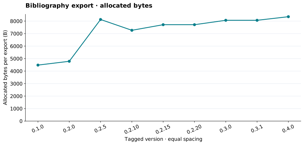
Allocated bytes, allocation count and live memory are three separate quantities. One large buffer can allocate more bytes than many small objects; many small objects cost more management work. Neither equals resident process memory. See Process memory.

Garbage collection

• The GC reclaims managed memory the program no longer needs; collecting it is work.

• GC time — measured collection time, in the same unit as the timing (BenchmarkTools).

• GC fraction — that time divided by elapsed time (Chairmarks).

Never merge the two.

• Zero recorded GC time in a short sample does not mean zero allocations — the collector may simply not have run.

• Do not add GC time to elapsed time; the elapsed interval already contains it.

Warm and cold code

• Julia compiles methods on first call.

• A warm benchmark measures repeated execution after preparation.

• A cold or first-call experiment must include the startup, loading or compilation boundary explicitly.

Warm latency says nothing about using YourPackage.

Flame graphs

• A call stack is the chain of calls leading to the current function.

• A flame graph aggregates many stacks into nested rectangles.

• Width — the selected weight (CPU samples, task samples or allocation bytes).

• Depth — the calling relationship. Horizontal position is not a timeline.

• A wide parent includes its descendants. Do not add parent and child percentages.

CPU, wall-time and allocation flame graphs look similar but weight different things. Read the metric, unit and legend first.

Comparability

Compare two numbers only when their measurement definitions and comparison keys agree. A run records the conditions so a consumer can check.

• Different OS, architecture, Julia threads or hardware make a comparison incomparable.

• A changed runtime or environment is a warning.

• A missing measurement stays missing. It never becomes an improvement.

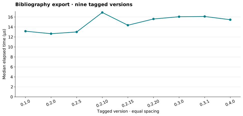
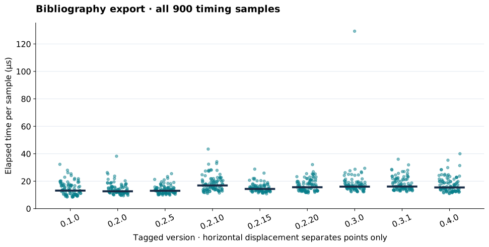
Recorded examples

One hundred samples per tag, Windows, Julia 1.13.0, one worker thread. Inputs match; the dependency stack evolves with the tags. Lower means less elapsed time.

Each dot is one sample; the dark marks are medians. Horizontal displacement only separates dots. Overlap and slow observations remain visible.

Julia allocation activity per operation. These values are neither retained heap size nor resident process memory. All nine points come from recorded measurements.

Next

• Collectors — what each tool records.

• Investigate a change — locate the cost with a profile.